Predicting oil recovery factor using dense and cascade neural networks
The question
Do the extra connections in cascade networks improve oil-recovery predictions?
Neural networks are a common way to estimate oil recovery quickly instead of running a full reservoir simulation. Cascade-forward networks add direct connections from the inputs and earlier layers to every later layer, and an earlier chemical-flooding study ranked one the most accurate of several models. We asked whether that design keeps an advantage over a standard dense network on a much larger, noisier dataset of 163,726 simulated polymer-flooding samples.
What we found
On held-out samples, the two networks achieved similar test R² values, which measure fit: 0.908 for the dense network and 0.906 for the cascade network, with identical average errors. The cascade network reached this result with 20 hidden neurons compared with 448 in the dense network, and both relied most on the averaged oil and water saturations.
Schematic overview
Changing the network connections and checking unseen simulated rows
Summarise the simulated flow state
Generate polymer-flooding simulations, then record seven quantities. Spatially varying pressure, fluid saturations, and polymer concentration are averaged to make table entries.
Compare two ways of connecting layers
A dense network passes information through successive layers. A cascade network also gives later layers direct access to inputs and earlier layers.
Keep test rows outside training
Add artificial noise, train the models on one portion of the table, and evaluate on held-out rows. Compare their prediction errors on that simulated-data task.
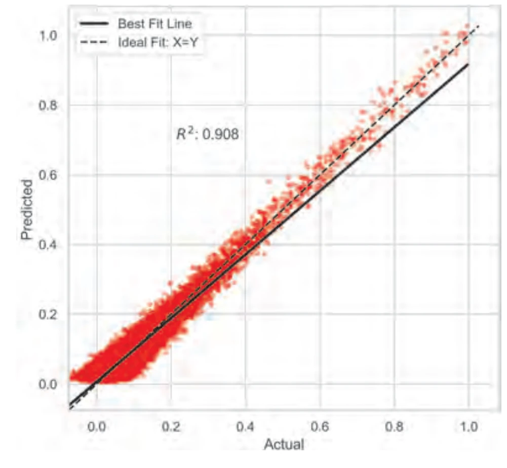
A held-out test of the dense network
Each red point compares the simulator’s recovery value on the horizontal axis with the network’s prediction on the vertical axis. The dashed diagonal marks exact agreement. The spread and fitted black line show the remaining mismatch.
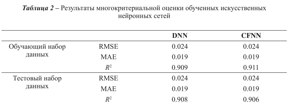
Both networks have nearly the same test scores
The lower block is the test set; the upper block is training. DNN means dense and CFNN means cascade. Both test columns report RMSE 0.024 and mean absolute error 0.019. Their R² values differ by just 0.002; this is not a percentage-accuracy score.
Figure details and test conditions
The dataset contains 163,726 synthetic rows, with Gaussian noise added. Thirty percent was held out for testing. R² describes fit relative to predicting the test-set mean, with 1 indicating perfect fit. The inputs include simulated flow-state summaries, not only initial rock and fluid properties. The two implementations also use different layer sizes, activations, and training algorithms, so this is not a controlled test of wiring alone.
Comparing dense and cascade networks
Data-driven proxy models can estimate oil recovery far faster than full reservoir simulations, and neural networks have been especially effective in this role. Two recurring designs are dense networks, which connect each layer only to the next, and cascade-forward networks, which also connect the inputs and every earlier layer directly to later layers. Those additional connections allow the cascade design to capture linear and nonlinear relationships together. In an earlier comparison for surfactant–polymer flooding, a cascade network trained with the Levenberg–Marquardt method was the most accurate of several models, with a 0.66% error.
That study, like others we reviewed, worked with far fewer cases than ours. We asked whether the cascade design keeps its advantage on a much larger and noisier dataset: 163,726 samples from a Buckley–Leverett polymer-flooding model.
The simulated inputs and prediction target
Each sample has seven inputs: permeability, porosity, oil viscosity, and the averaged pressure, oil and water saturation, and polymer concentration from the simulation. The target is the oil recovery factor, the fraction of the original oil recovered. Models trained on the noise-free data reached near-perfect scores, so we added Gaussian noise with a standard deviation of 30% of each variable’s own spread. We then held out 30% of the samples for testing.
Accuracy and model size
The dense network had three hidden layers of 256, 128, and 64 neurons, with 43,265 trainable parameters, and was trained in TensorFlow. The cascade network needed only two hidden layers, of 15 and 5 neurons, and was trained in MATLAB with the Levenberg–Marquardt method. On the test set, both had the same root-mean-square error (0.024) and mean absolute error (0.019). Their R² values were 0.908 and 0.906. Permutation tests showed that both relied most on oil and water saturation, and least on viscosity.
Scope of the study
The saturation inputs come from the simulation itself; before noise was added, recovery was perfectly correlated with water saturation (1.00). The task is therefore to estimate recovery from a simulated flow state rather than to forecast it from properties known before injection. Testing on real datasets with more reservoir parameters is the next step. These are the same two networks as in our nine-model benchmark, described here in detail.